Getting Started with Spatial & Time Analysis Toolbox
Installation:
1. Unpack the spatialbox.zip into directory
$matlabroot$\work\spatialbox (recommended), where $matlabroot$ is the path of
the Matlab[1] installation path.
Execution
a) Run the RUN.BAT
file by double-clicking its name in the Windows XP explorer window, or manually
by: Start à Run à type: run.bat and press Enter.
Otherwise, if the user wishes to work with Matlab and start the toolbox
from the Matlab desktop:
b) Start Matlab by
matlab.exe or Start à Programs and select Matlab 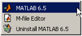
Note: It is
possible to run the toolbox without loading Java Virtual Machine (JVM)
environment of Matlab. The memory consumption of Matlab without JVM is much
lower and it is recommended if the user encounters Out of Memory errors or slow
performance. In order to run Matlab in the ‘text mode’ change the command line
of the icon to matlab –nojvm or Start à Run à matlab -nojvm
Change the path to the directory with the toolbox, or add the toolbox’s directory to the Matlab path
a) Change working directory >> cd c:\matlab6p5\work\spatialbox
or
b) Add
path by >> addpath
c:\matlab6p5\work\spatialbox
Check that Matlab recognizes the
toolbox by typing
>>
help spatialbox
If the output does not look like:
SPATIALBOX Application M-file for spatialbox.fig
FIG = SPATIALBOX launch spatialbox GUI.
SPATIALBOX('callback_name', ...) invoke the named callback.
Then please, check the path or
repeat the above steps.
It is also possible to add the
Spatial Toolbox directory to the Matlab path with GUI (only under JVM
environment) by: 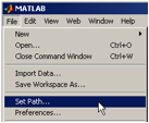 and then
 ![]()
Getting started
If the main window (Figure
1) is not on the screen, run the toolbox by >> spatialbox from the Matlab
desktop.
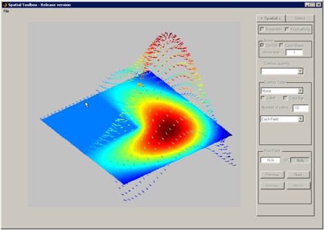
Figure 1: Spatial toolbox GUI - main window
At the top-right corner
there are Menu (File, Window) and the toolbar icon (Load files), in the center
there is a main axes and on the right-hand side there are GUI controls.
The Spatial Toolbox
operation begins with loading the data. The data could be loaded as InsightÒ[2] *.vec or *.v3d files, by
File à Load Vector File.
The user can press the ![]() button and then select the folder that
includes the data files from the window, shown in Figure 2, or type the name of
the folder instead of the default path. There is an option to double-click the
.. in the list of files box, or double click the name of the directory within
the list in order to get the files in the subdirectory. *.vec files are listed
as a default, and the user can check checkbox ‘switch to .v3d’ in the in order to see the list of *.v3d files.
button and then select the folder that
includes the data files from the window, shown in Figure 2, or type the name of
the folder instead of the default path. There is an option to double-click the
.. in the list of files box, or double click the name of the directory within
the list in order to get the files in the subdirectory. *.vec files are listed
as a default, and the user can check checkbox ‘switch to .v3d’ in the in order to see the list of *.v3d files.
When the list of files is
shown (see Figure 3), user might use on the
selection options:
- If one file is selected, when the Load button is pressed, all the
files from the selected file and up to the last file, listed in the box,
will be loaded into Matlab
- If two files are selected, with CTRL button and mouse clicks, then
all the files between these two are loaded.
- If user selects manually more than 2 files, with CTRL and clicks, or
with SHIFT and extending the selection, then only the selected files are
loaded.
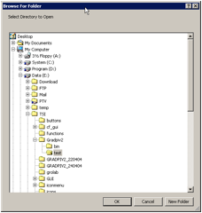
Figure 2: List of the directories to choose the path of the VEC or V3D files
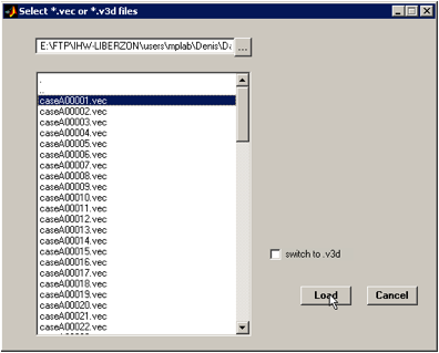
Figure 3: Selection of the files from the listbox. One, two with CTRL, or many with CTRL or SHIFT options are possible. Press LOAD button to finish the selection.
Press Load button to finish
the selection. The Spatial Toolbox reads the vector files, initializes the
toolbox default variables and calculates several flow quantities. This part
might take from several seconds to a few minutes, depending on the length of
the selected series and the size of each vector map[3].
This part is re-implemented
(since the last release of the Spatial Toolbox on April 16.), by using uigetdir
function.
Note: for the Spatial and Time Analysis Toolbox, the
order of the selected files is not important, the user might pick the last file
first and after that the first file. However, during the loading procedure, the
files will be automatically sorted in the ascending order of their file names.
This default sorting procedure is due to the original goal of the toolbox is
Time Series Analysis, where Time Series is presumably recorded with PIV in some
kind of sequence.
Operating
Instructions
When at least one vector file is selected, the
default window looks like in the following Error! Reference source not
found..
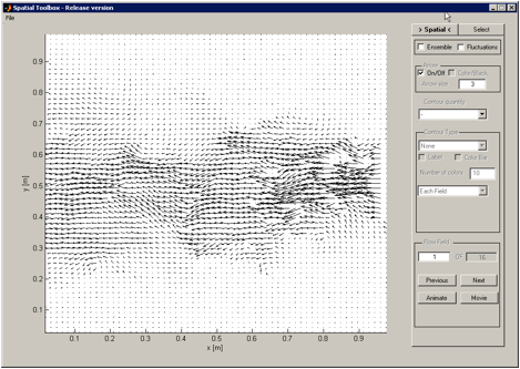
Figure 4: Default window, arrows, GUI controls, main
axes.
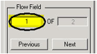
Navigation
- Navigation is done by the next/previous
buttons, which displays next/previous maps accordingly
- To jump to specific map,
enter number of the map in edit box, followed by Enter:
Available options:
The user
might choose between one of the large set of various combinations to present
its data: arrows in black or in color. The color of arrows could represent any
one of the available quantities for that particular mode. The arrows could be
on top of the contour map of the selected quantity, and contour could be as
color patterns, bounded, or unbounded (smooth view), color or black contour
lines. Below, in the working example, we show some of the combinations.
Controls:
Arrows
§
On /Off – shows / hides arrows
§
Color /Black – if turned on, arrows will be colored
according to the current quantity
Contour Quantity
The user can choose the quantity
that will be displayed on the screen. There are four main sets of
quantities (we can call them 4 modes). The switch between the modes is done
with two checkboxes ![]() :
:
1.
Instantaneous mode (not one of the checkboxes is checked on): the list of
quantities is:
![]()
2.
Ensemble averaged mode (only Ensemble checkbox is checked on), ensemble
averages of the instantaneous quantities, the list is:
![]()
3.
Fluctuations mode (only the Fluctuations checkbox is checked on)![]()
4.
Turbulent quantities mode (both checkboxes are checked
on), the list is:
![]()
Contour type
Available contour types are:
§
Flood - smooth color patches, no sharp boundaries
§
Color Line - only
color boundaries, according to the color map of the selected quantity.
§
Flood + Line – color patches, with sharp boundaries
§
Black Line – only boundaries of the contours
There are several examples
given below to show some of the available arrow and contour combinations:
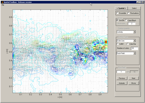
Figure 5: Instantaneous velocity field (arrows) and the
instantaneous vorticity
field in color-line
contour mode. Color bar
is added and the number of contour levels is set to be 25.
Control of contour levels (i.e. colors)
The user can
manually enter number of contour levels (or number of colors), by entering the
desired number in the edit box: ![]() and pressing Enter.
and pressing Enter.
The number of colors
(default or manually set) defines the number of contour levels of the selected
quantity, but in one of four modes (contour modes):
§
Each Field – the contour is automatically updated to
each presented map limits (min and max) and distributed evenly into number of
contour levels (i.e. number of colors)
§
All to Display – the currently presented map defines
the contour levels for all forthcoming maps, unless other option is selected.
If the user changes the quantity, the limits are updated, but still will be
constant for all forthcoming views.
§ All Fields – the contour levels are defined by the maximum and minimum values of the selected quantity from the whole selected dataset. This is very powerful option, that allows one to compare the values visually, when not even one value will be out of the defined color set (which is possible to happen in manual or All to Display modes). However, one should realize that in order to determine the absolute maximum and minimum values, the whole dataset has to be calculated at least once. For example, All Fields of the vorticity demands the calculation of gradients in both directions of the selected dataset (which could be really long for the Time-Resolved PIV).
Manual - the user
can select the maximum and minimum level of the color to be shown, the
selection could be symmetric by entering the same positive and negative values
or anti-symmetric, if different values are used.
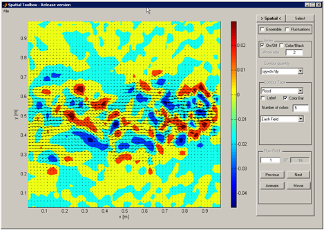
Figure 6: Instantaneous velocity field (longer arrows,
set to 3), Flood contour type of the rate-of-strain component, number of
contour levels set to 3 to emphasize strong positive and negative regions.
Animation
The user can run the animation of the successive maps, with all the visualization properties that were selected before, by pressing Animation button. The first map is the current map (that could be manually entered in the edit box) and pressing again the Animation button stops the animation at any map. Otherwise the animation will continue up to the last map.
During the animation, the movie is NOT stored in the memory. The user should operate Movie button in the same way as Animation button, but in addition, the user will be prompted to type in the file name of the AVI file. The Windows AVI video file (uncompressed, default frame-per-second rate of 15 fps) is saved, when the last map is reached, or the Movie button is pressed again (i.e. released).
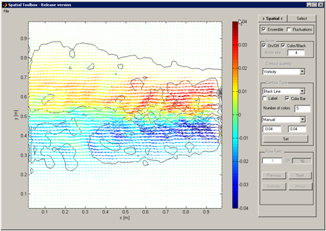
Figure 7: Ensemble averaged velocity field, shown by
arrows. The color of
the arrows and the sharp boundaries are of the average vorticity field, the number of contour levels
is set to 5, and the color is distributed symmetrically by manual set of
contour levels between –0.04 and 0.04 [1/sec].
Selecting region of interest for Time Toolbox or Distribution analysis
1) In order to select data, move to ‘select’ tab, where selection tools are placed:
![]()
Figure 8: Switching to selection tab
2) Selection Tools – in selection tab, the following selection tools are present (see Figure 9)
2.1 General
description
- Only one type of selection is allowed, for example points can’t be selected with region.
- In order to quit selection mode, after region/points are selected, press middle mouse button or 3rd mouse button.
- When ‘Reset’ button is pressed all selections are cleared.
- When ‘Spatial’ tab is pressed, all selections are cleared.
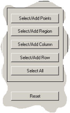
Figure 9: Selection tools
2.2 Select/Add points – allows to select single/multiple points from the map (see Figure 10)
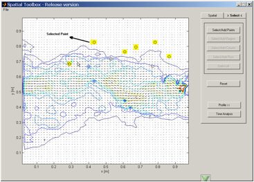
Figure 10: Selecting points
2.3 Selecting Region(s)
- In order select region press ‘Add region’
- Adding two or more regions: there is restriction to select only regions that have at least one side equal, and ends of the side lie on the same line:
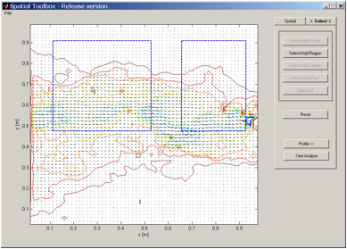
Figure 11: Selecting regions
2.4 Selecting Rows/Column
- Press ‘Add Row’ or ‘Add Column’ to select the entire row/column:
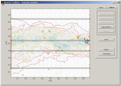
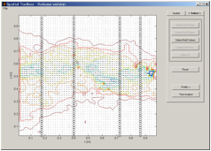
Figure 12: Selecting rows (left) or columns (right).
2.4 Select All
- Pressing ‘Select All’ will select the entire map (see Fig.6)
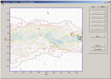
Figure 13: Selecting the entire map.
Profile analysis
- After selection is done, press ‘Profile’ button in order to show Distribution window:
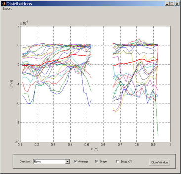
Figure 14: Distribution window, with the Average distribution added to the plot (thick red line). The case is for the two disconnected regions.
Available options:
- Direction (Rows/Columns) – changes one of the axis to x/y respectively
- Swap X-Y – changes between axes (Fig.8)
- Single – all the data in the selected region of interest (rows or columns or regions or all) is shown in spatial distribution along rows or along columns (i.e. X or Y profile per row or column).
Average – when turned on, red line presenting average of quantities is shown.
File Menu options:
- Export-> Figure: Export to Matlab figure allows one to use Plot Edit options of Matlab
- Export->CSV: Allows user to export select file name, for saving data in CSV format.
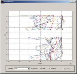
Figure 15: Distirbution with axes
swaped (rotated 90 degrees) by checking 'Swap X-Y'.
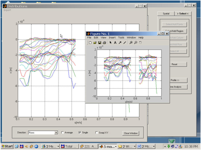
Figure 16: The example of the Export to
Figure output.
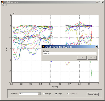
Figure 17: When Export to CSV file is chosen, user is prompted to type the file name.
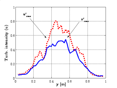
Figure 18: The Export to Figure allows the user to copy one curve from the figure into another, add text, arrows, etc. and change all the visual style of the figure.
Time Analysis Toolbox - Matlab toolbox for the High Image Frame Rate PIV analysis
The only necessary step to transfer data to the Time Toolbox is the selection of the region of interest. As it is described above, the selection could be a set of points, rows, columns, regions or the whole map. When the selection is done, the Time Analysis button is pressed.
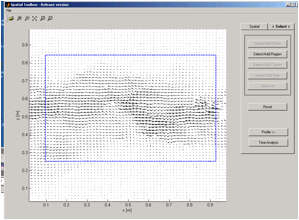
Figure 19: Selection of the region of interest
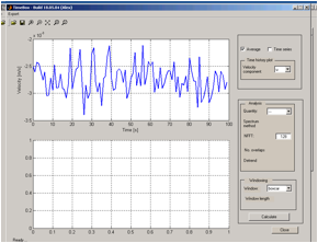
Figure 20: First window of the Time Toolbox, default plot is spatial averaged time history of the u velocity (from left to right).
The possible selections in Velocity Component list are instantaneous and fluctuating velocity components from the left to right (u), from the top to bottom (v) and in case of stereoscopic PIV data it includes also the out-of-plane component w.
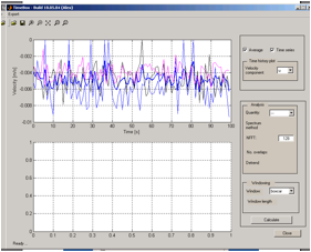
Figure 21: Time history of the selected point, operated by checking the Time Series checkbox. Note that Average is checked too, and it is emphasized by thick blue line.
Depends on the two checkboxes, the user might choose to see only pointwise time history and/or its spatial average. In addition, the user can plot the time history of the fluctuation velocities, same as the instantaneous for the three components.
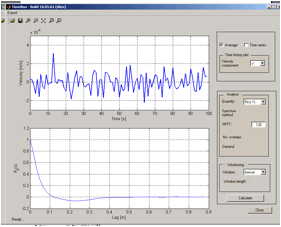
Figure 22: An example of the lateral correlation, Rii relates to the selected velocity component (i.e. if u is selected it is Ruu, from the left to the right) and k1 refers to the rows direction (from the top to the bottom).
The available quantities are: the autocorrelation function in time and space (longitudinal and lateral), and the respective spectrums – the frequency spectrum and two wave-number spectra. For more details and definitions, please see the definitions and formulae in the contract attachment. The quantities have to be operated on the fluctuations in order to obtain meaningful results.
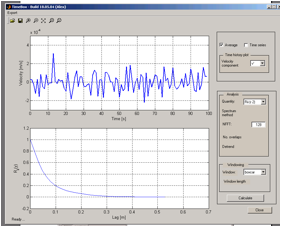
Figure 23: An example of the longitudinal correlation function, in this case it is Rvv in k2 direction.
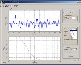
Figure 24: An example of the wave-number spectra.
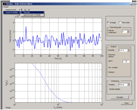
Figure 25: Each one of the axes could be independently exported or saved into Matlab figure or comma separated file.
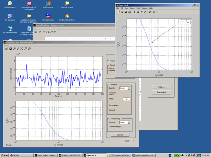
Figure 26: Export to Matlab figure allows one to use Plot Edit options of Matlab.
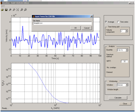
Figure 27: For each comma separated file, a unique file name is used.